No 6. Synthesis
Now it is time to put the pieces together and see what pictures emerge. What do these patterns tell us about host specificity?
Phylogenetic Visualization
IMNGS analysis
To dig just a little deeper, we screened our DA ASVs against the IMNGS database. IMNGS hosts a curated database of short-read sequences scraped from the International Nucleotide Sequence Database Collaboration (GenBank, DDBJ and EMBL). The database is rebuilt monthly and at the time of this analysis, contained 271,237 samples. IMNG is really designed to screen full-length 16S rRNA sequences and is not ideal for shorter reads. This is because the database is built from short reads, and different studies target different regions of the gene. For example, if we get no hits to an ASV it could mean the organisms it came from has really not been detected before or that it is in the database but is represented by a different 16S region. So take these data with a grain of salt.
IMNGS is not a high-throughput system. User may only submit a maximum of 10 sequences per query and this can (and will) take weeks to run. So choose your ASVs carefully.
IMNGS will return a lot of useful data for each query sequence. All we were interested in here was the number of hits, but there much more really useful data here. Among other data products, IMNGS returns report tables that tally the number of samples that were positive for the presence of query-like sequences for each sample category—categories like shrimp gut metagenome and seawater metagenome. Each category has a number of short-read samples, which could originate from a single study or multiple studies.
A report includes values for several percent identity cutoff values. We set a minimum threshold at 97% so our reports have values for 97 and 99%. You can set the threshold as low as 90%.
IMNGS provides three such reports based on the abundance of your query sequence.
An SRA-derived sample is considered positive if the query-like sequences sum up to more than 0% of the total number of sequences in that sample (i.e. any abundance).
An SRA-derived sample is considered positive if the query-like sequences sum up to more than 0.1% of the total number of sequences in that sample (i.e. excluding rare abundances).
An SRA-derived sample is considered positive if the query-like sequences sum up to more than 1% of the total number of sequences in that sample (i.e. including only dominant OTUs).
We report data from 97% cutoff identity and 0.1% of total reads in a sample. I think this is a little confusing so let me explain by example. In the tree below, ASV398 is most closely related to an Alphaproteobacteria associated with the toxic benthic marine dinoflagellate, Ostreopsis ovata. We retrieved this sequence during the BLASTn analysis discussed above. Anyway, ASV398 was screened against IMNGS and returned 2460 hits. This means that at 97% identity, 2460 samples had an ASV398-like sequence comprising greater than 0.1% of a given samples total number of sequences. If for example we increase the percent identity to 99% the number of sample hits drops to 138. If instead we look at the 0% report (97% identity), the number of sample hits increases to 6323.
Sullam lifestyle categories
We also compared the final list of top hits to the Sullam et. al. paper, specifically Table S1 from that paper. Because this paper was published in 2012, there were many sequence hits in our db that did not appear in the original paper. However, for those that did, we added the Sullam lifestyle category designations to the tree metadata.
Putting the pieces together
We took all of these data and used iTOL to visualize the tree. For each top hit, we added the isolation source/natural host information, taxonomic affiliation, and Sullam lifestyle category. We also overlaid the number of hits to the IMNGS database for each ASV.
To view a full, interactive version of the tree go this iTOL page.
Figure 3
You can pan around and zoom in on this tree. Double-clicking will zoom in on an area.

Inferring Lifestyle Category
We used the tree to infer the lifestyle category of each ASVs based on the closest relatives in their clade. This was not a quantitative, but rather a user guided determination. Aside from MetaMetaDb (discussed above) we are not aware of any tool currently available to quantitatively assess habitat preference of a 16S rRNA sequence.
For simplicity we focused on three lifestyle catagories (though we have seven categories in the tree). Our reasoning—again based on the work of Sullam et. al.—was that fish intestines contain microbes that are generalists and possibly of environmental origin (what they eat, where they live), microbes that are there because fish are animals with guts, and microbes that are there because fish are fish and have a physiology and evolutionary history that select specific organisms. Sullam et.al. were also looking at fish from different habitats (freshwater, estuary, marine) and tropic levels (carnivores, herbivores, omnivores) while our study was more narrow in scope.
- fish associated: ASVs most closely related to sequences from the intestinal tract of marine fish.
- animal associated: ASVs most closely related to sequences from other animals, including one freshwater fish, other vertebrates, and a few non-marine invertebrates.
- generalists: ASVs most closely related to sequences are widespread and possibly from the environment. By and large these are marine or marine-like (e.g., hypersaline mats, saline lakes) in origin including sediments, water, and potential prey (algae, plants, coral, sponge). However there are some leaves in the tree from non-marine environments (e.g., activated sludge) that we grouped in the environmental category.
Assessing habitat specificity.
We combined these habitat predictions with the results of the BLASTn analysis, scan of the IMNGS database, Sullam lifestyle categories, etc. and put it all in one editable table. So if you disagree with a habitat prediction, you can feel free to change it.
Table S6
habi_tab <- read.table("DATA/PHYLOSEQ/TABLES/INPUT/habitat_specificity.txt",
                       header = TRUE, sep = "\t", check.names = FALSE)
# order by habitat and host enriched
habi_tab2 <- habi_tab[order(habi_tab$habitat_code, habi_tab$Enriched), ]
#habi_tab <- habi_tab[, -2] #delete code column
da_asvs_counts <- as.data.frame(taxa_sums(da_asvs))
colnames(da_asvs_counts) <- c("total_reads")
# make rownames a column
da_asvs_counts <- cbind(ASV = rownames(da_asvs_counts), da_asvs_counts)
temp_table <- merge(da_asvs_counts, blast_tab, by = "ASV",
                    all = TRUE, sort = FALSE)

summ_table <- merge(temp_table, habi_tab2, by = "ASV",
                    all = TRUE, sort = FALSE, no.dups = TRUE)

summ_table <- summ_table[-c(22, 26, 27, 28, 29, 31)]
summ_table <- summ_table[c(1, 22, 23, 2, 24, 4, 3, 5, 6, 7, 8, 18, 19, 20,
                           9, 10, 11, 12, 13, 14, 15, 16, 17, 21, 25)]

datatable(summ_table, rownames = FALSE,
          colnames = c(
            "ASV", "Putative habitat", "Enriched", "Total reads",
            "Taxon", "Num perfect hits", "Top hit acc", "% identity",
            "Isolation source", "Nat host", "Common name", "Collection year",
            "Country", "PubMed ID", "Alignment length", "Mismatches",
            "Gap opens", "Q. start", "Q. end", "S. start", "S. end",
            "Evalue", "Bit score", "Num IMNGS hits", "Sullam lifestyle"),
          editable = TRUE, caption =
            htmltools::tags$caption(
              style = "caption-side: bottom; text-align: left;",
              "Supplementary Table 6: ",
              htmltools::em("Assessing habitat specificity.")),
          extensions = "Buttons",
          options = list(columnDefs =
                           list(list(className = "dt-center",
                                     targets = c(1, 2, 3, 4, 5,
                                                 6, 7, 8, 9, 10))),
                         dom = "Blfrtip", pageLength = 5,
                         lengthMenu = c(5, 10, 25, 60),
                         buttons = c("csv", "copy"),
                         scrollX = TRUE, scrollCollapse = TRUE))
write.table(summ_table, "DATA/PHYLOSEQ/TABLES/OUTPUT/SUPP/Table_S6.txt",
sep = "\t", col.names = c(
"ASV", "Putative habitat", "Enriched", "Total reads",
"Taxon", "Num perfect hits", "Top hit acc", "% identity",
"Isolation source", "Nat host", "Common name",
"Collection year", "Country", "PubMed ID", "Alignment length",
"Mismatches", "Gap opens", "Q. start", "Q. end", "S. start",
"S. end", "Evalue", "Bit score", "Num IMNGS hits",
"Sullam lifestyle"),
row.names = FALSE, quote = FALSE, fileEncoding = "UTF-8")This table also scrolls horizontally.
NR Indicates Not Recorded. Four ASVs had numerous hits at 100% identity. We did not include top hit data for these ASVs.
Description of table headings
- ASV: ASV id.
- Total Reads: Total reads of ASV.
- Putative habitat: Our habitat designation based on the analyses.
- Enriched: Which of the five herbivorous reef fish the ASV was enriched in.
- Taxon: Taxonomic classification of the ASV.
- closest db match: Host or environment of top hit.
- % identity: Percent identity of top hit.
- subject acc Accession number of top BLAST hit
- IMNGS hits: Number of hits to the IMNGS database. Value indicates the number of samples that scored a hit to an ASV.
- Sullam lifestyle: Lifestyle category as defined by Sullam et. al., 2012. NLC indicates no hit to the Sullam db.
- num perfect hits Number of 100% BLAST matches out of 50 top hits.
Summary of habitat preference
Now we can summarize the data for each lifestyle category. This table was constructed in a text file and read into R.
Table 1
habi_summary <- read.table("DATA/PHYLOSEQ/TABLES/INPUT/Table_1.txt",
                           header = TRUE, sep = "\t", check.names = FALSE)

datatable(habi_summary,
          rownames = FALSE, editable = TRUE,
          caption = htmltools::tags$caption(
            style = "caption-side: bottom; text-align: left;",
            "Table 1: ", htmltools::em("Summary of habitat specificity.")),
          extensions = "Buttons",
          options = list(columnDefs = list(list(className = "dt-center",
                                                targets = c(1, 2, 3, 4, 5))),
                         dom = "Brti", buttons = c("csv", "copy"),
                         scrollX = TRUE, scrollCollapse = TRUE))
Taxa by Host
So we know that Host X is enriched for some ASV from taxa Y. Is this part of a larger pattern or an isolated case? For a given taxonomic group and rank, what proportion of total reads (from all ASVs) were found in a particular host species? At some point it would be nice if this were an interactive step, but for now we must modify the code below to look at different taxa. This example will look at the family Desulfovibrionaceae (Deltaproteopbacteria)
Proportion of total reads for a given taxon & rank
# Change this to select different taxa
calc_tax_prop <- subset_taxa(mergedGP, Family == "Desulfovibrionaceae")
calc_tax_prop
## phyloseq-class experiment-level object
## otu_table() OTU Table: [ 71 taxa and 5 samples ]
## sample_data() Sample Data: [ 5 samples by 3 sample variables ]
## tax_table() Taxonomy Table: [ 71 taxa by 8 taxonomic ranks ]sample_sums_by_taxa <- sample_sums(calc_tax_prop)
total_taxa_reads <- sum(sample_sums_by_taxa)
sample_sums_by_taxa <- as.data.frame(sample_sums_by_taxa)
sample_sums_by_taxa$proportion <-
(sample_sums_by_taxa$sample_sums_by_taxa /
total_taxa_reads) * 100
colnames(sample_sums_by_taxa) <- c("total taxa reads", "Proportion")
sample_sums_by_taxa$Proportion <- round(sample_sums_by_taxa$Proportion,
digits = 2)
total_taxa_reads_int <- as.integer(total_taxa_reads)
sample_sums_by_taxa## total taxa reads Proportion
## AcCoe 133418 64.51
## AcTra 52223 25.25
## ScTae 805 0.39
## SpAur 5742 2.78
## SpVir 14643 7.08Great. Looks like there are 71 Desulfovibrionaceae ASVs and the majority (> 90%) of the reads are from Acanthurus. This is interesting. We can do this with any taxa we wish.
Proportion of total reads for Cyanobacteria
So lets do this to also look at the proportion of Cyanobacteria reads by host species.
# Change this to select different taxa
calc_tax_prop_Cyan <- subset_taxa(mergedGP, Phylum == "Cyanobacteria")
calc_tax_prop_Cyan
## phyloseq-class experiment-level object
## otu_table() OTU Table: [ 484 taxa and 5 samples ]
## sample_data() Sample Data: [ 5 samples by 3 sample variables ]
## tax_table() Taxonomy Table: [ 484 taxa by 8 taxonomic ranks ]sample_sums_by_taxa_Cyan <- sample_sums(calc_tax_prop_Cyan)
total_taxa_reads_Cyan <- sum(sample_sums_by_taxa_Cyan)
sample_sums_by_taxa_Cyan <- as.data.frame(sample_sums_by_taxa_Cyan)
sample_sums_by_taxa_Cyan$proportion <-
(sample_sums_by_taxa_Cyan$sample_sums_by_taxa_Cyan / total_taxa_reads_Cyan) * 100
colnames(sample_sums_by_taxa_Cyan) <- c("total taxa reads", "Proportion")
sample_sums_by_taxa_Cyan$Proportion <- round(sample_sums_by_taxa_Cyan$Proportion,
digits = 2)
total_taxa_reads_Cyan_int <- as.integer(total_taxa_reads_Cyan)
sample_sums_by_taxa_Cyan## total taxa reads Proportion
## AcCoe 9177 12.73
## AcTra 22781 31.61
## ScTae 26681 37.02
## SpAur 6283 8.72
## SpVir 7157 9.93There were a total of 484 Cyanobacteria ASVs across 72079 reads.
DA ASV by Host
At this point we know which ASVs are enriched in which host species, the lineage of those ASVs, and something about where else these sequences have been detected in nature. Next we would like to know the proportion of total reads for each ASV that is found in each host species. We start with a summary table of these data.
Proportion of total ASV reads per host species
# calculate the averages and merge by species
# grab the da_asv ps object & merge by samples
daASV_mergedGP_BAR <- merge_samples(da_asvs_full, "Sp")
#daASV_SD_BAR <- merge_samples(sample_data(da_asvs_full), "Sp")
# calculate percent proportion
daASV_AVG <- apply(t(otu_table(daASV_mergedGP_BAR)), 1, function(x) x / sum(x))
# transpose
daASV_t_AVG <- t(daASV_AVG)
daASV_t_AVG_df <- as.data.frame(daASV_t_AVG)

######################
# choose columns of interest
da_ASV_tax <- habi_tab[c("ASV", "Taxon", "Putative_habitat")]
da_ASV_tax2 <- da_ASV_tax[, -1]
rownames(da_ASV_tax2) <- da_ASV_tax[, 1]

######################
# combine based on ASV column
daASV_work <- merge(daASV_t_AVG_df, da_ASV_tax2, by = 0, sort = FALSE)

rownames(daASV_work) <- daASV_work[, 1]
daASV_work[, 1] <- NULL
#daASV_work

# then make column row.names
daASV_work2 <- cbind(ASV = rownames(daASV_work), daASV_work)
# melt the df
# wide to long format?
daASV_work3 <- melt(daASV_work2, value.name = "ASV")
## Warning in melt(daASV_work2, value.name = "ASV"): The
## melt generic in data.table has been passed a data.frame
## and will attempt to redirect to the relevant reshape2
## method; please note that reshape2 is deprecated, and
## this redirection is now deprecated as well. To continue
## using melt methods from reshape2 while both libraries are
## attached, e.g. melt.list, you can prepend the namespace
## like reshape2::melt(daASV_work2). In the next version, this
## warning will become an error.colnames(daASV_work3) <- c("ASV", "Taxon", "Putative_habitat",
"Sample", "Proportion")
daASV_work3$Proportion <- round(daASV_work3$Proportion, digits = 4)
datatable(daASV_work3,
rownames = TRUE, editable = FALSE,
caption =
htmltools::tags$caption(
style = "caption-side: bottom; text-align: left;", "Table 8: ",
htmltools::em("DA ASV sample proportion.")),
extensions = "Buttons",
options = list(columnDefs = list(list(className = "dt-center",
targets = c(1, 2, 3, 4, 5))),
dom = "Blfrtip", pageLength = 5,
lengthMenu = c(5, 10, 50, 100, 300),
buttons = c("csv", "copy"), scrollX = TRUE,
scrollCollapse = TRUE))write.table(daASV_work3, "DATA/PHYLOSEQ/TABLES/OUTPUT/prop_ASV_reads_by_host.txt",
sep = "\t", row.names = FALSE, quote = FALSE)Now that we have a list of DA ASVs and their assigned habitat preference, we want to create a R object that organizes these in some logical fashion. We can then use this object to order subsequent graphs and tables. So lets order the ASVs by putative habitat preference and then by the host species in which that ASV was enriched. Seems reasonable enough? Depending on the R command, some objects need to be in ascending order, others in descending order.
asv_order <- c("ASV450", "ASV165", "ASV395", "ASV284", "ASV56",
               "ASV6", "ASV359", "ASV128", "ASV127", "ASV91",
               "ASV374", "ASV151", "ASV323", "ASV398", "ASV224",
               "ASV39", "ASV34", "ASV12", "ASV32", "ASV250",
               "ASV43", "ASV54", "ASV9", "ASV5", "ASV49", "ASV8",
               "ASV41", "ASV18", "ASV7", "ASV90", "ASV29", "ASV98",
               "ASV23", "ASV30", "ASV226", "ASV48", "ASV70", "ASV1",
               "ASV14", "ASV298", "ASV82", "ASV75", "ASV69", "ASV57",
               "ASV20", "ASV15", "ASV2", "ASV268", "ASV114", "ASV234",
               "ASV174", "ASV60", "ASV17", "ASV22", "ASV159", "ASV44",
               "ASV25", "ASV21", "ASV35")
asv_order_rev <- rev(asv_order)
Lets see if we can overlay all of this information in one “easy” to understand plot. The first thing is to do is plot the proportion of reads for a given ASV from each host species.
Graph for proportion of total ASV reads per host species
daASV_work3$ASV <- as.character(daASV_work3$ASV)
daASV_work3$ASV <- factor(daASV_work3$ASV, levels = unique(daASV_work3$ASV))
daASV_work3$ASV <- factor(daASV_work3$ASV, levels = asv_order)
Next, we created a bar plot of read proportion by host species for each ASV. And save a copy to the DATA/PHYLOSEQ/FIGURES/ directory.
Proportional bar chart
#Bar charts
ASV_bar <- ggplot(daASV_work3, aes_string(x = "ASV", y = "Proportion",
                                          fill = "Sample"),
                  environment = .e, ordered = TRUE,
                  xlab = "x-axis label", ylab = "y-axis label")

ASV_bar <- ASV_bar +
  geom_bar(stat = "identity", position = position_stack(reverse = TRUE),
           width = 0.95) +
  coord_flip() +
  theme(aspect.ratio = 2 / 1)

ASV_bar <- ASV_bar +
  scale_fill_manual(values = samp_pal)

ASV_bar <- ASV_bar +
  theme(axis.text.x = element_text(angle = 0, hjust = 0.95, vjust = 1))

ASV_bar <- ASV_bar +
  guides(fill = guide_legend(override.aes = list(colour = NULL),
                             reverse = FALSE)) +
  theme(legend.key = element_rect(colour = "black"))

ASV_bar <- ASV_bar +
  labs(x = "Host species", y = "Proportion (% total reads)",
       title = "ASV Proportion by host species")

ASV_bar <- ASV_bar +
  theme(axis.line = element_line(colour = "black"),
        panel.grid.major = element_blank(),
        panel.grid.minor = element_blank(),
        panel.border = element_rect(colour = "black", fill = NA, size = 1))
ASV_bar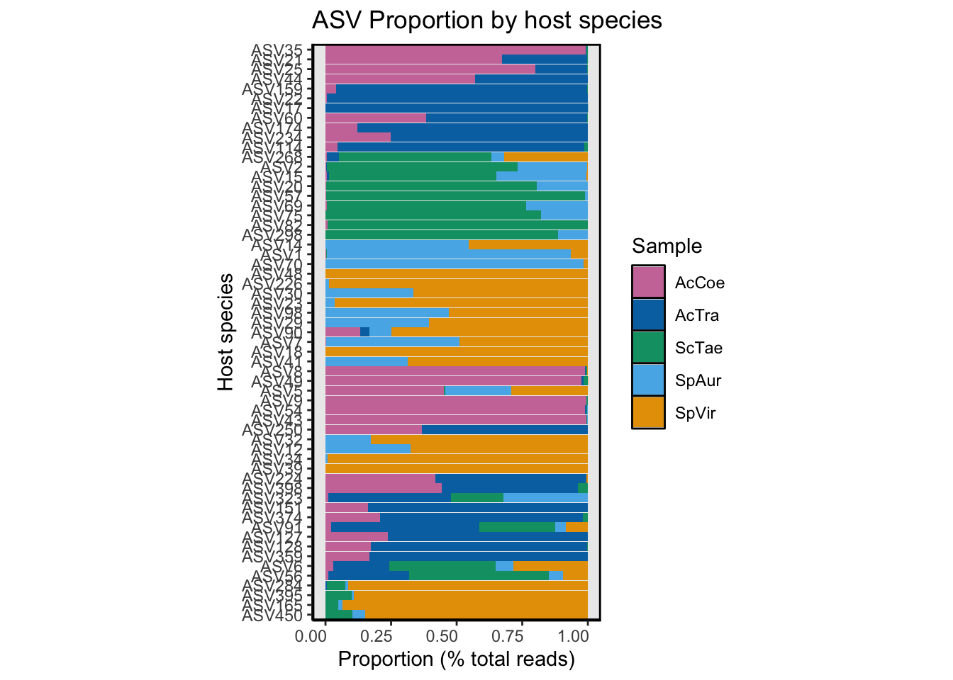
Heatmap
Figure 4 (mostly)
# Heatmap
library(ComplexHeatmap)
library(circlize)
library(heatmap3)
library(gdata)
fig4_heat <- as.data.frame(t(otu_table(da_asvs)))
# Convert habi_table to df and store in new variable
fig4_tax <- as.data.frame(habi_tab2)
# eliminate 1st column so can combine based on row names
fig4_tax_tab <- fig4_tax[, -1]
# Make new row.names from original table
rownames(fig4_tax_tab) <- fig4_tax[, 1]
# Reorder
fig4_tax_tab <- fig4_tax_tab[c(4, 2, 3, 1, 5, 6, 7, 8)]
# Select columns
fig4_tax_tab <- fig4_tax_tab[c(1:4)]

# Combine the two df by rowname If the matching involved row names,
# an extra character column called Row.names
# is added at the left, and in all cases the result has ‘automatic’ row names.
fig4_heatmap2 <- merge(fig4_tax_tab, fig4_heat, by = 0, all = TRUE)

fig4_heatmap <- subset(fig4_heatmap2, select = -c(Row.names))
rownames(fig4_heatmap) <- fig4_heatmap2[, "Row.names"]
# make rownames a column
fig4_heatmap <- cbind(ASV = rownames(fig4_heatmap), fig4_heatmap)

fig4_heatmap$ASV <- factor(fig4_heatmap$ASV, levels = rev(asv_order))
fig4_heatmap <- fig4_heatmap[order(fig4_heatmap$ASV), ]
# combine the columns to make one name
fig4_heatmap$ID <- paste(fig4_heatmap$ASV, fig4_heatmap$Taxon,
                         fig4_heatmap$Putative_habitat,
                         fig4_heatmap$Enriched, sep = "_")
# delete the original columns
fig4_heatmap2 <- fig4_heatmap[-c(1:5)]
# reorder
fig4_heatmap2 <- fig4_heatmap2[c(6, 1, 2, 3, 4, 5)]
rownames(fig4_heatmap2) <- fig4_heatmap2[, 1]
fig4_heatmap2 <- fig4_heatmap2[-1]

####Define Colors
taxa_colors <- unlist(lapply(row.names(fig4_heatmap2), function(x) {
  if (grepl

     # generalists
               ("Alphaproteobacteria", x)) "#000000"
  else if (grepl("Pirellulaceae", x)) "#000000"
  else if (grepl("Rubritaleaceae", x)) "#000000"
  else if (grepl("Flavobacteriaceae", x)) "#000000"

   # fish/animal
  else if (grepl("Desulfovibrionaceae", x)) "#0072b2"
  else if (grepl("Lachnospiraceae", x)) "#f0e442"
  else if (grepl("Erysipelotrichaceae", x)) "#009e73"
  else if (grepl("Ruminococcaceae", x)) "#e69f00"
  else if (grepl("Bacteroidales", x)) "#d55e00"
  else if (grepl("Fusobacteriaceae", x)) "#56b4e9"
  else if (grepl("Vibrionaceae", x)) "#cc79a7"

  # other
  else if (grepl("Family_XIII", x)) "#808080"
  else if (grepl("Mollicutes", x)) "#808080"
  else if (grepl("Brevinemataceae", x)) "#808080"
  else if (grepl("Peptostreptococcaceae", x)) "#808080"
}))

habitat_colors <- unlist(lapply(row.names(fig4_heatmap2), function(x) {
  if (grepl
               ("fish", x)) "#808080"
  else if (grepl("animal", x)) "#000000"
  else if (grepl("generalist", x)) "#808080"
  #else if (grepl("undetermined", x)) "#000000"
}))
heatColors <- cbind(taxa_colors, habitat_colors)
colnames(heatColors)[1] <- "Taxa"
colnames(heatColors)[2] <- "Habitat"
### SAVE/display heatmap
col <- colorRampPalette(bias = 1, c("#000033", "#66CCFF"))(16)
pdf(file = "DATA/PHYLOSEQ/FIGURES/OUTPUT/Figure_4B.pdf")
heatmap3(fig4_heatmap2, cexRow = 0.5, cexCol = 1,
         margins = c(3, 13), RowSideColors = heatColors, scale = "row",
         Colv = NA, Rowv = NA, revC = TRUE, balanceColor = FALSE, col = col)
invisible(dev.off())
heatmap3(fig4_heatmap2, cexRow = 0.5, cexCol = 1,
         margins = c(3, 13), RowSideColors = heatColors, scale = "row",
         Colv = NA, Rowv = NA, revC = TRUE, balanceColor = FALSE, col = col)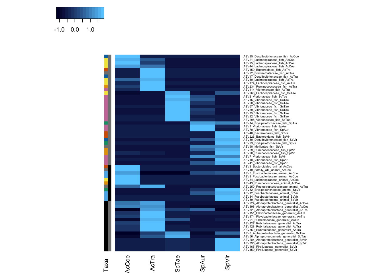
Combine the two charts.
Either do outside R or figure out a way to ‘bolb’ the heatmap. grid::grid.grab seemed promising.
ASVs & Host Trait Correlation?
To test whether intestinal microbes were associated with a) phylogenetic history and/or b) foraging ecology of each herbivore, we used a series of simple and partial Mantel tests. Because we expected the relationships to potentially differ for putative resident symbionts vs. ingested environmental generalist microbes, we constructed separate dissimilarity matrices for host- and environment-associated ASVs. These matrices were constructed using the vegan package in R and were based on Bray-Curtis dissimilarity of Hellinger transformed data. The ecological dissimilarity matrix was based on the behavioural data collected to quantify herbivore trophic niche space.
The phylogenetic dissimilarity matrix was based on a phylogenetic tree of the five fish species used in this study. We constructed the tree using cytochrome oxidase subunit 1 (COI) genes retrieved from NCBI’s Nucleotide Database. Clustal Omega was used to align sequences (default settings for DNA). We then used Jalview to manually curate and trim the final alignment to 593 bp. This alignment contained COI genes from n = 5 Scarus taeniopterus, 22 Sparisoma aurofrenatum, 21 Sparisoma viride, 28 Acanthurus coeruleus, and 23 Acanthurus tractus. We used members of the Gerridae (2 Eucinostomus and 4 Gerres) as the outgroup. We used RAxML and the GTR model for tree computation and the GAMMA rate model for likelihoods. The tree was then transformed into a distance matrix using the cophenetic function in R.
detach("package:phyloseq", unload=TRUE)
library(ape)
library(picante)
library(ggtree)
library(tidytree)
library(treeio)
# Get phylogenetic data ------------------
# Read newick tree ------------------
tree <- read.tree("DATA/PHYLOSEQ/TABLES/INPUT/MANTEL_TEST/item_orders.txt")
#ggtree(tree) + geom_tiplab(color = "blue")

host_tree <- knitr::include_graphics("images/collapse_tree.svg",
                                     dpi = 300)
host_tree
Next, we pruned the tree to one member of each species, removed the outgroup, and changed the names to species names.
d <- matrix(nrow = 1, ncol = 5)
colnames(d) <- c("HM379826_Acanthurus_coeruleus",
               "LIDM544-07_Acanthurus_tractus",
               "MXIV480-10_Scarus_taeniopterus",
               "JQ841390_Sparisoma_aurofrenatum",
               "JQ839595_Sparisoma_viride")
tree.p <- prune.sample(phylo = tree, samp = d)
#plot(tree.p)
# Change the names to species names
tree.p$tip.label[1] <- "Sparisoma_aurofrenatum"
tree.p$tip.label[2] <- "Sparisoma_viride"
tree.p$tip.label[3] <- "Scarus_taeniopterus"
tree.p$tip.label[4] <- "Acanthurus_tractus"
tree.p$tip.label[5] <- "Acanthurus_coeruleus"
plot(tree.p)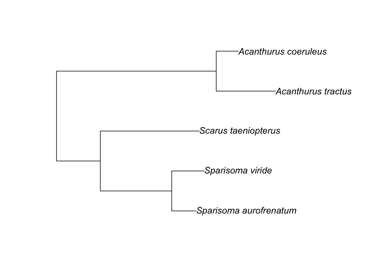
We then transformed the tree into a distance matrix and generated a dendrogram.
#Transform tree into a distance matrix
trx <- cophenetic(tree.p)
#that works but I need these in alphabetical order by species
T <- dist(cophenetic(tree.p))
ordering <- sort(attr(T, "Labels"))
T.mat <- as.matrix(T)[ordering, ordering]
T  <- as.dist(T.mat)
#plot cluster of distance matrix
cluster_phylo <- hclust(T, method = "ward.D")
plot(cluster_phylo, main = "Phylogenetic clustering",
     xlab = "Host species", ylab = "Distance",
     sub = "hellinger/bray-curtis/ward")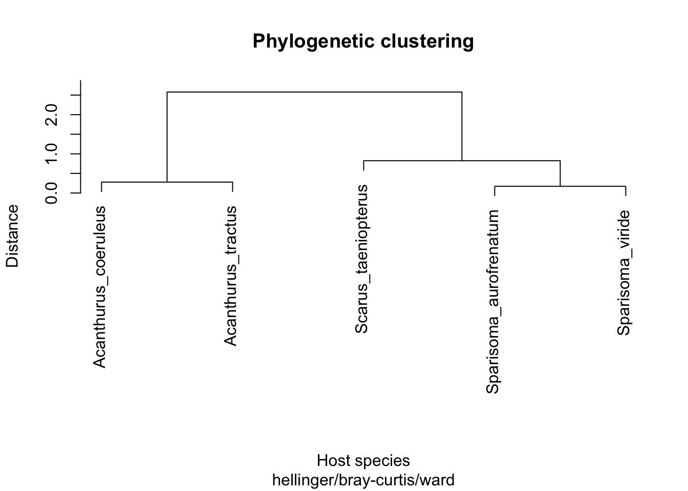
Next we grab the ecological data and standardize the variables so that they have similar weights.
First, rescale quantitative traits to be in the range 0 to 1 and then devide by the number of diet categories to have similar influence as the diet variables. Then rescale all ‘non diet’ traits to have similar influence to the diet traits by dividing by the number of diet categories divided by the number of categories for each substrate characteristic. Now combine into a single data frame for analysis get averages for each species.
all_traits <- read.csv(
  "DATA/PHYLOSEQ/TABLES/INPUT/MANTEL_TEST/Mean_bite_characteristics.csv",
  header = TRUE
  )
ids <- all_traits[, 1:2]

quant_traits_std <- decostand(all_traits[, 3:4], "range") / 10

Mean_prop_mark_on_substrate_std <- all_traits[, 5] / (10 / 2)
prop_vertical_std <- all_traits[, 6] / (10 / 2)
prop_concave_std <- all_traits[, 7] / (10 / 3)
prop_convex_std <- all_traits[, 8] / (10 / 3)

all_traits_std <- cbind(quant_traits_std,
                      Mean_prop_mark_on_substrate_std,
                      prop_vertical_std, prop_concave_std,
                      prop_convex_std,
                      all_traits[, 9:18]
                      )

mean_traits <- aggregate(all_traits[, 3:18],
                         by = list(all_traits$Species), mean)
traits <- mean_traits[, 2:17]
rownames(traits) <- as.vector(mean_traits[, 1])
Fish_species <- as.vector(mean_traits[, 1])
And begin with a Hellinger transformation of Ecological traits.
traits_trans <- decostand(traits, method = "hellinger")
traits_dist <- vegdist(traits_trans, method = "bray")
cluster_traits <- hclust(traits_dist, method = "ward.D")
plot(cluster_traits,
     labels = Fish_species, main = "Ecological traits",
     xlab = "Host species", ylab = "Distance",
     sub = "hellinger/bray-curtis/ward")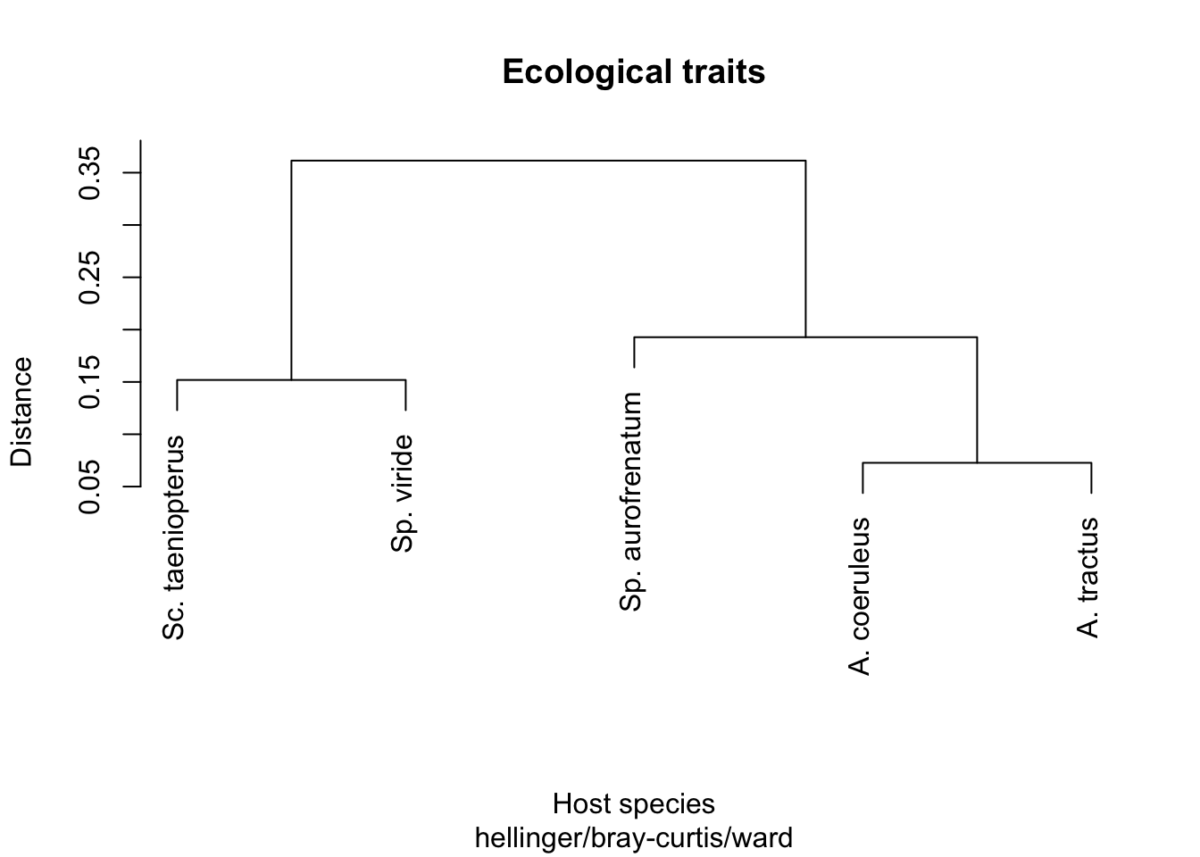
So, is ecological data correlated with phylogeny?
# Is ecological data correlated with phylogeny
mantel(traits_dist, T, method = "pearson", permutations = 9999)
##
## Mantel statistic based on Pearson's product-moment correlation
##
## Call:
## mantel(xdis = traits_dist, ydis = T, method = "pearson", permutations = 9999)
##
## Mantel statistic r: 0.4816
## Significance: 0.175
##
## Upper quantiles of permutations (null model):
## 90% 95% 97.5% 99%
## 0.593 0.654 0.751 0.817
## Permutation: free
## Number of permutations: 1190K, looks like there is no correlation between ecological data and phylogeny. Next, we looked at differentially abundant ASVs split into host-associated vs environmentally associated
asv4 <- read.delim(
  "DATA/PHYLOSEQ/TABLES/INPUT/MANTEL_TEST/2_da_asv_merged_fish.txt",
  header = T
  )
asv5 <- read.delim(
  "DATA/PHYLOSEQ/TABLES/INPUT/MANTEL_TEST/2_da_asv_merged_animal.txt",
  header = T
  )
asv_host <- rbind(asv4, asv5)

# Merge the fish and animal datasets together
# Transpose dataframe
asv_host_t <- data.frame(t(asv_host[-1]))
colnames(asv_host_t) <- asv_host[, 1]

library(vegan)
# Create dendrogram based on similarity in asv

Fish_species <- as.vector(colnames(asv_host[2:6]))
Gut_contents <- sqrt(asv_host_t[])
#Try hellinger transformation
Gut_contents <- decostand(asv_host_t, method = "hellinger")
Gut_dist_host <- vegdist(Gut_contents, method = "bray")
cluster_gut_host <- hclust(Gut_dist_host, method = "ward.D")
plot(cluster_gut_host, labels = Fish_species, main = "Host-associated ASVs",
     xlab = "Host species", ylab = "Distance", sub = "hellinger/bray-curtis/ward")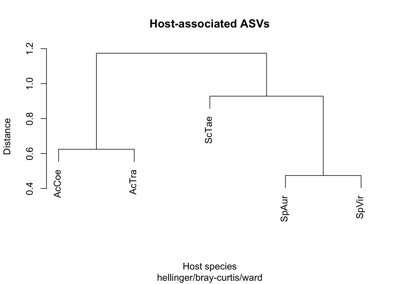
So is the distance matrix (based on host associated ASVs) correlated with ecological data or phylogeny?
mantel(Gut_dist_host, T, method = "pearson", permutations = 9999)##
## Mantel statistic based on Pearson's product-moment correlation
##
## Call:
## mantel(xdis = Gut_dist_host, ydis = T, method = "pearson", permutations = 9999)
##
## Mantel statistic r: 0.8448
## Significance: 0.0083333
##
## Upper quantiles of permutations (null model):
## 90% 95% 97.5% 99%
## 0.556 0.711 0.754 0.820
## Permutation: free
## Number of permutations: 119Yes, highly correlated with phylogeny…
mantel(Gut_dist_host, traits_dist, method = "pearson", permutations = 9999)##
## Mantel statistic based on Pearson's product-moment correlation
##
## Call:
## mantel(xdis = Gut_dist_host, ydis = traits_dist, method = "pearson", permutations = 9999)
##
## Mantel statistic r: 0.2511
## Significance: 0.25833
##
## Upper quantiles of permutations (null model):
## 90% 95% 97.5% 99%
## 0.490 0.585 0.662 0.752
## Permutation: free
## Number of permutations: 119# Not associated with ecological traits…but not associated with ecological traits.
What about the distnace matrix based on environment associated ASVs? Is it correlated with ecological data or phylogeny?
asv6 <- read.delim(
  "DATA/PHYLOSEQ/TABLES/INPUT/MANTEL_TEST/2_da_asv_merged_environmental.txt",
  header = T)
# Transpose dataframe
asv_env_t <- data.frame(t(asv6[-1]))
colnames(asv_env_t) <- asv6[, 1]

# Create dendrogram based on similarity in asv
Fish_species <- as.vector(colnames(asv6[2:6]))
Gut_contents <- sqrt(asv_env_t[])
#Try hellinger transformation
Gut_contents <- decostand(asv_env_t, method = "hellinger")
Gut_dist_env <- vegdist(Gut_contents, method = "bray")
cluster_gut_env <- hclust(Gut_dist_env, method = "ward.D")
plot(cluster_gut_env, labels = Fish_species,
     main = "Environment-associated ASVs",
     xlab = "Host species", ylab = "Distance",
     sub = "hellinger/bray-curtis/ward")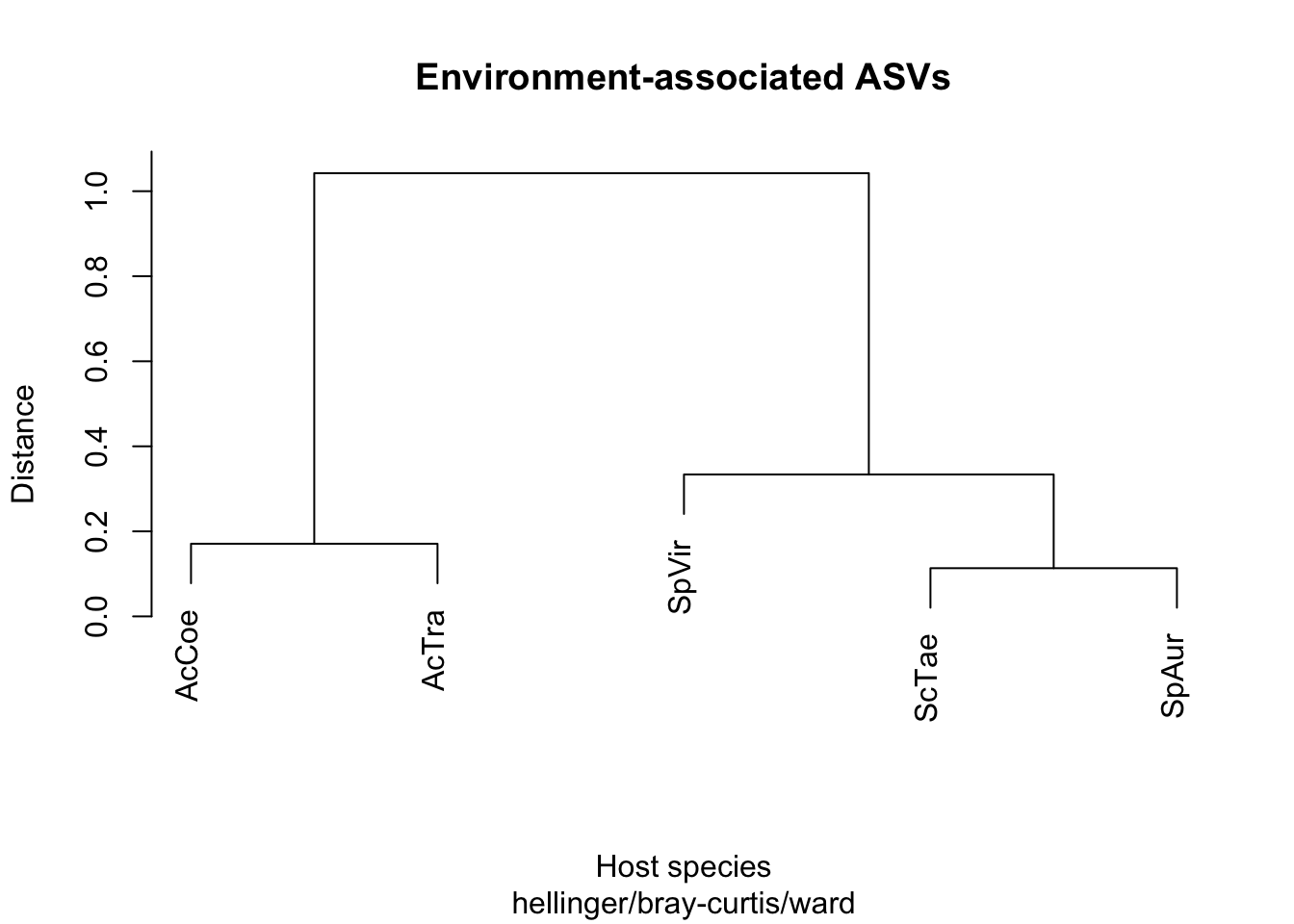
mantel(Gut_dist_env, T,
       method = "pearson", permutations = 9999
       )
##
## Mantel statistic based on Pearson's product-moment correlation
##
## Call:
## mantel(xdis = Gut_dist_env, ydis = T, method = "pearson", permutations = 9999)
##
## Mantel statistic r: 0.8313
## Significance: 0.075
##
## Upper quantiles of permutations (null model):
## 90% 95% 97.5% 99%
## 0.455 0.862 0.893 0.931
## Permutation: free
## Number of permutations: 119# Marginally significant correlationDoesn’t look correlated with phylogeny…
mantel(Gut_dist_env, traits_dist,
       method = "pearson", permutations = 9999
       )
##
## Mantel statistic based on Pearson's product-moment correlation
##
## Call:
## mantel(xdis = Gut_dist_env, ydis = traits_dist, method = "pearson", permutations = 9999)
##
## Mantel statistic r: 0.5963
## Significance: 0.083333
##
## Upper quantiles of permutations (null model):
## 90% 95% 97.5% 99%
## 0.531 0.690 0.765 0.788
## Permutation: free
## Number of permutations: 119…or ecological data.
We could also do partial Mantel tests.
mantel.partial(Gut_dist_env, T, traits_dist,
               method = "pearson", permutations = 9999
               )
##
## Partial Mantel statistic based on Pearson's product-moment correlation
##
## Call:
## mantel.partial(xdis = Gut_dist_env, ydis = T, zdis = traits_dist, method = "pearson", permutations = 9999)
##
## Mantel statistic r: 0.7734
## Significance: 0.091667
##
## Upper quantiles of permutations (null model):
## 90% 95% 97.5% 99%
## 0.497 0.829 0.871 0.914
## Permutation: free
## Number of permutations: 119mantel.partial(Gut_dist_env, traits_dist, T,
method = "pearson", permutations = 9999
)##
## Partial Mantel statistic based on Pearson's product-moment correlation
##
## Call:
## mantel.partial(xdis = Gut_dist_env, ydis = traits_dist, zdis = T, method = "pearson", permutations = 9999)
##
## Mantel statistic r: 0.4022
## Significance: 0.15
##
## Upper quantiles of permutations (null model):
## 90% 95% 97.5% 99%
## 0.516 0.632 0.830 0.839
## Permutation: free
## Number of permutations: 119But again, no significance detected…